Graphs
Contents
Graphs#
Theory#
A graph \(G\) of order \(o\) will be fully described by a square adjacency matrix \(\mathcal{A}\in\mathbb{M}_{o\times o}(\mathbb{R})\) and a state vector \(\mathcal{S}\in\mathbb{R}^{o}\).
The adjacency matrix contains the weights \(w(e_{i,j})\) of the edges (from the vertex \(v_i\) to \(v_j\) in this case). The particular case of \(w(e_{i,j})=0\) indicates that their is no edge going from \(v_i\) to \(v_j\).
The state vector contains the states \(s(v_i)\) of the vertices \(v_i\).
The neighborhood \(N(v)\) of a vertex \(v\) is the set of vertices which are adjacent to it. Thanks to the linear algebra description of graphs, there is a simple way to obtain a vector containing the weighted sum of the states present in the neighborhood of every vertex of a graph.
We can also define the n-th neighborhood \(N_n(v)\) of a vertex as the set of vertices which are at a distance \(n\) of \(v\).
Examples#
The Graph class can be instantiated with two inputs: an adjacency matrix and a state vector both in the form of nested arrays.
import gra

graph = gra.Graph([ # adjacency matrix
        [0, 1, 1, 1],
        [1, 0, 1, 1],
        [1, 1, 0, 1],
        [1, 1, 1, 0]
    ],[ # state vector
        [1],
        [0],
        [0],
        [0]
    ])
Graph objects have three atributes:
adjacency_matrix( an instance of the SparseTensor class of TensorFlow )state_vector( an instance of the Tensor class of TensorFlow )dtype( a numpy data type object: np.int32 or np.float32 )
and eight methods:
.plot(): plots the graph.evolve(rule): evolves the graph according therule.order(): returns the order of the graph.diameter(): returns the diameter of the graph.clone(): returns a copy of the graph, this allows to use rules without modifying the original graph.to_igraph(): returns an igraph object.to_networkx(): returns a networkx object.to_mathematica(): returns a string corresponding to a Mathematica compatible version of the graph
In the case of binary graphs \([s(v)\in \{0,1\}\;\forall v]\), plots are such that:
“alive” vertices \([s(v)=1]\) are colored purple,
“dead” vertices \([s(v)=0]\) are colored orange.
graph.plot()
Graphs with a different ordering of vertices are equivalent. This equivalence can be checked with ==.
graph == gra.Graph([ # adjacency matrix
        [0, 1, 1, 1],
        [1, 0, 1, 1],
        [1, 1, 0, 1],
        [1, 1, 1, 0]
    ],[ # state vector
        [0],
        [0],
        [1],
        [0]
    ])
True

